|
|
X-Ray tomography
|
|
X-ray radiation is a unique tool for diagnosis, because diffraction and refraction are minimal in this case, and hence the simple ray optics model can be employed. In terms of this model the inverse problem of tomography can be reduced to solving linear integral equations (the Radon transform). In the case of full-range data, hundreds of efficient methods can be proposed to address the inverse problems arising in x-ray tomography. By full-range data we mean that the object can be illuminated from all directions and the detectors can be placed on all sides around it. Figure 1 shows a real tomogram of a seashell. Cross sections 1 to 6 obtained in Z=const planes are shown in the right-hand panel of the figure.
|
|
|
| Figure 1 Tomogram of a seashell: (a) X-ray projection image; (b) reconstructed cross-sections. |
|
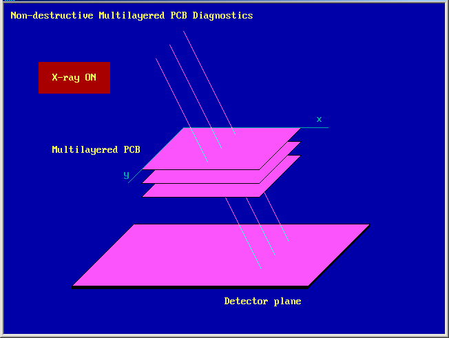
In the case of limited-range data the solution of inverse problem is generally non-unique. It makes no sense trying to solve it by inventing new algorithms. The only way is to use supplementary information about the object examined. The obvious information that the sought-for function ρ(r) describing the attenuation is positive is of no particulat help. The situation changes essentially if the supplementary information is the fact that the 3D object examined consists of a set of layers. Figure 2 shows the scheme of a tomographic experiment involving the diagnosis of a five-layer printed circuit board (PCB)
.
|
|
|
| Figure 2 Scheme of the tomography experiment |
|
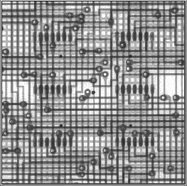
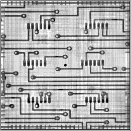
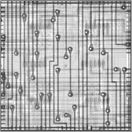
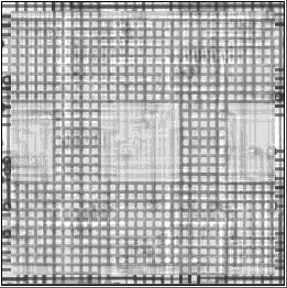
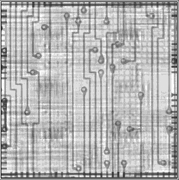
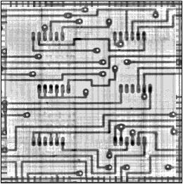
Figure 3 shows the reconstructed images of the five-layer printed circuit board. The board examined has the size of 50×50 cm, the width of conductors is 400 μm, and the inter-layer spacing is 300 μm. The fragments shown in the figure are 5 × 5 cm in size.
|
|
|
| Figure 3: (a) - Input data (an image registered by the detectors); (b)-(f) reconstructed images of the metal layers |
|
Mathematically the inverse problem in the case of tomographic diagnosis of layered objects reduces to solving an ill-conditioned set of linear equations with a large number of unknowns. [1]
|
|
References
|
|
1. Bakushinsky A., Goncharsky A. Ill-posed problems: Theory and applications. Kluwer Acad Publ., DORDRECHT/Boston/, London, 1994.
|
![[MSU]](../img/msu.jpg)